EQUATIONS
The qm view's simple equations specify a variety of complex phenomena including "relativistic phenomena,"
"inertia," and "gravity." These equations and related phenomena are explained briefly below, and other pages on
this website explain them in greater detail. Most of the website's pages fit on a computer screen, but this page
and the Facts page are among
the exceptions. The below explanations include examples showing how the equations are used to predict and explain
phenomena, including the illusion of Earth's pull on our bodies and less obvious phenomena, such as the bending
of light paths around massive bodies, and the small changes in the rates of our clocks and our aging due to our
constantly changing motions and locations.
Premises (and phenomena) responsible for the equations
In the qm view, all forms of mass/energy, including all things that science has been able to
sense, are comprised of oscillations of a quantum medium. "Energy quanta" (e.g. photons) are oscillations
that move through the qm at the speed of light. They can have energies that range from less than 1E−15
times the energy of a photon of visible light to greater than 1E15 times a visible photon's energy.
In the qm view, these oscillations can form self-contained systems of oscillations that can have any
speed through the qm less than the speed of the oscillations through the qm. Within a small system of oscillations
(e.g. electron or quark), the oscillations move very short distances before being absorbed or reflected or
otherwise interacting with other mass/energy in the system.
In the qm view, all the particles of the current standard model of particle physics are systems of
oscillations of the qm. Presently, the nature of the oscillations and systems of oscillations is unknown, and
the reason for assuming them is that the consequences of this assumption explain a wide variety of important
phenomena that have not had a common, plausible explanation (e.g. constant light speed, c, the huge internal
energies in joules of small masses in kilograms, and the "inertia" and "weight" of
mass/energy systems).
Even small masses are comprised of large numbers of oscillations that must be moving in all directions within
a body. For example, an electron contains the equivalent of 1E5 uv-photon oscillations, and the motions
of the oscillations within the system must be essentially isotropic when the system is at rest in the qm.
However, when a system of oscillations is moving through the qm, the speeds of the oscillations moving within
the system are no longer isotropic in the system. This is important because it causes a variety of phenomena
including the slowing of time in the system and a foreshorting of the system along lines parallel to its
direction of motion through the qm. The causes are explained below. They are all consequences of the following
two premises.
Premise I:
A quantum medium is present everywhere in the universe and the mass/energy of the universe consists of
oscillations of the medium. Individual energy quanta (e.g. photons) are propagated through the medium with
a constant absolute speed, ca, when not impeded directly by mass/energy (e.g. air, water) or
indirectly by nearby large concentrations of mass/energy (e.g. stars, galaxies), according to
Premise II.
Note: The qm view and supporting evidence indicate that
electrons, quarks, and other "particles" having rest mass are all dynamic systems of oscillations in the qm.
This view is consistent with the thinking of Paul Dirac, who showed that electrons and other particles can be
excitations of the ether medium that Maxwell assumed was necessary for the propagation of electromagnetic
energy. The nature of the oscillations or excitations in the medium is presently unknown. With the exception
of Premise II, the quantum medium does not impede the motion of any form of
mass/energy through the medium, as discussed here.
Premise II:
Every concentration of mass/energy (e.g. person, planet, star, galaxy) decreases the speed at which energy
(e.g. photons) is propagated through the quantum medium in its vicinity. The speed, cag, is a simple
function of the magnitude of the mass/energy (kga), the distance (LS) from the mass/energy, and
Newton's gravitational constant (2.47E−36   kg
kg s s ) (i.e. 6.674E−11/c)
as explained below.
cag = (1 + (m·G / ) (i.e. 6.674E−11/c)
as explained below.
cag = (1 + (m·G / ) ) ) )
Note: The cag equation specifies a gradient around every massive body
of the rate at which energy can be transfered through the qm. How massive bodies cause the photon-slowing gradients
is presently unknown.
Units of measurement
The equations discussed below involve units of time, distance, mass, force, and other physical quantities,
so we need to define the most important units. The physical standard of speed in the qm view is the absolute
speed of light, ca, where "absolute" means the speed through the quantum medium as opposed to
speed relative to a source or observer of light, and also means the light is not slowed either directly by
mass/energy in its path (e.g. air) or indirectly by concentrations of mass/energy (e.g. stars).
Most physicists today realize that the seconds determined by atomic clocks depend on the clocks' distances from
Earth's center of mass, and they know that a clock's motions can affect the elapsed time on the clock.
If two atomic clocks are initially together and synchronized, and then one clock is taken on a high-speed round trip
(or is taken to a location with different gravity), the clocks will keep different times and will no longer be
synchronized when brought together again. The qm view explains why the physical standards of time, distance, and
mass (i.e. the "standard" clocks, meter bars, and masses kept by governments in carefully controlled environments)
are constantly changing: The physical standards depend on their velocities through the qm and their distances
from massive bodies (e.g. sun, moon). These velocities and distances are constantly changing due to Earth's
motions in the cosmos.
In the qm view, the primary unit of time is the absolute second, sa, a second according to an ideal or perfect
atomic clock at rest in the qm and not influenced by any concentration of mass/energy. In this theoretical
environment, the clock will evolve at its fastest possible rate. Clocks moving through the qm or near concentrations
of mass/energy specify virtual seconds, s, that are longer time durations than 1 sa. The qm view,
including the equations below, explains how the various rates of virtual seconds recorded by clocks can be converted
into the rate of absolute seconds that specifies the universal advancement of time.
The primary unit of distance in the qm view is the absolute light-second, LS, which is a fixed
distance — as opposed to a virtual light-second, , which is illusory.
One LS is the distance that light travels with absolute speed, ca, through the qm in 1 sa.
One is the
distance between any two points in an inertial reference frame where the round-trip travel time for a light signal
between the two points is two seconds, according to clocks in the reference frame. One LS is a longer distance
than 1 . An absolute meter, ma, is equal to 1 LS divided by 299792458
(1 ma ≈ 1 LS / 3E8) and is longer than a virtual meter, m, which is
1 / 299792458 and also illusory. (A standard meter bar in a controlled, stable,
local environment is illusory in the sense that it appears to represent a fixed length, but actually changes length
due to changes in absolute velocity, orientation, and location relative to massive systems.)
In the qm view, the primary unit of mass and/or energy (i.e. mass/energy) is the
absolute kilogram, kga, which can be defined in terms of the Planck constant and photon oscillation
frequencies in cycles per absolute second, sa. One kga is a fixed amount of mass/energy as opposed to a
virtual kilogram, kg, specified by a standard kilogram mass, which changes absolute mass due to changes
in its absolute velocity and location relative to massive systems.
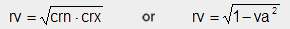
Relative speeds of light, cr, crn, and crx
The speed of light relative to a body or reference frame is represented by the symbol cr.
This speed depends on the absolute velocity, va, of the body or reference frame through the qm and the
direction of the light through the medium. The minimum speed of light, crn, and the maximum speed of light,
crx, relative to the body or reference frame, are specified by the following equations, where the units of
the variables are ca, the maximum speed of light through the qm.
Example: If a spaceship is moving through the qm with absolute velocity of .2 ca, the minimum and
maximum speeds of light relative to the ship are
crn=(1−.2)=.8 ca
and crx=(1+.2)=1.2 ca.
These minimum and maximum speeds of light are in the direction of the ship's absolute velocity and in the opposite
direction respectively. The speeds of light relative to the ship in all other directions are between crn and crx.
(For further clarification click here.)
Physical change ratio, rv
The physical change ratio, rv, for a body or reference frame is a function of crn and crx or the absolute
velocity, va, of the body or reference frame, as follows.
Example: An atomic clock, a quartz crystal clock, and an oscillating flywheel clock aboard a spaceship moving
through the qm with absolute velocity va=.1 ca evolve at a rate of
rv=(.9 ·1.1) =.994... or
rv=(1−.1 =.994... or
rv=(1−.1 )=.994...
times their rate when at rest in the qm. This ratio also specifies physical changes in masses and distances
in the spaceship. If the ship has a mass of 100000 kga and a length of 50 ma when at rest in
the qm, its mass will be (100000 / .994...) kga, its length will be
(50 ·.994...) ma (if its length is parallel to its direction of absolute velocity),
and its width and height will be its at-rest width and height. )=.994...
times their rate when at rest in the qm. This ratio also specifies physical changes in masses and distances
in the spaceship. If the ship has a mass of 100000 kga and a length of 50 ma when at rest in
the qm, its mass will be (100000 / .994...) kga, its length will be
(50 ·.994...) ma (if its length is parallel to its direction of absolute velocity),
and its width and height will be its at-rest width and height.
Page 9 of this website provides evidence that Earth's absolute velocity through the quantum medium is probably
low, which indicates that rv on Earth is close to 1. The evidence indicates that the sun is moving with a velocity
of about .0012 ca through the quantum medium (assuming that an observer at rest in the quantum medium
would see an isotropic pattern of cosmic microwave background radiation). Earth's rotation and revolution
around the sun do not significantly change our velocity through the qm, and rv on Earth is about .9999992.
Bodies with very high speed motion on Earth may have lower rv values. For example, the electrons moving in cathode
ray tubes can have speeds of .1 ca and rv=.994..., and particles in large
accelerators can have speeds of .99999998 ca and rv=.0002.
Virtual relative velocity, vBC, and virtual physical change ratio, rBC
When two spaceships or reference frames, B and C, have constant absolute velocities, vBa and
vCa, through the qm in the same or opposite directions, observers in the ships or frames observe
a virtual velocity of B relative to C, vBC, that depends upon their absolute velocities, as shown
in the below-left equation. (The observed vBC depends on the observers' assumption that the speed of light
in their ship or frame is constant, c.)
The observed relative velocity, vBC, is always less than the absolute relative velocity, vBCa=vBa-vCa,
when vBa and vCa are not zero. This virtual relative velocity is used in the below-right equation to calculate
the virtual physical change ratio, rBC, between B and C. The observed slowing of clocks and changes in
length and mass in the other ship or frame are functions of rBC.
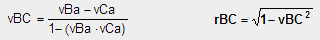
Example 1: Two hypothetically identical spaceships, B and C, are passing close to one another.
Time aboard the ships is kept by atomic clocks, and the times are displayed so they can be observed aboard
the other ship. Ship B has an absolute velocity vBa=.6 ca, and ship C has an absolute velocity
vCa=.8 ca in the same direction. Therefore, the absolute relative velocity of B relative to C
is vBCa=(.6−.8)=−.2 ca. Their observed virtual relative
velocity specified by the left equation is
vBC=(.6−.8) / (1−(.6·.8))=−.3846 c.
This virtual relative velocity vBC results in the virtual physical change ratio
rBC=(1−(−.3846))=.9230.
Therefore, observers on a ship observe that the clocks on the other ship run at .923 times the rate of their
clocks, and they observe that the length of the other ship is .923 times the length of their ship.
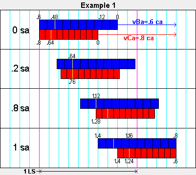
Example 2: Spaceships, B and C are passing one another.
Ship C has absolute velocity vCa=.8 ca, and B has absolute velocity vBa=.6 ca
in the opposite direction. Their absolute relative velocity is vBCa=(.6+.8)=1.4 ca.
Their observed virtual relative velocity specified by the left equation is
vBC=(.6−(−.8)) / (1−(.6·−.8))=.9459 c.
This virtual relative velocity vBC results in the virtual physical change ratio
rBC=(1−.9459)=.324.
Therefore, observers on a ship observe that the clocks on the other ship run at only .324 times the rate of
their clocks, and they observe that the other ship is only .324 times as long as their ship.
In both examples above, the observers on both spaceships agree on the virtual relative velocities between their ships.
Also in both cases, the observers on the ships all observe that the other ship is foreshortened and that its clocks
are running slow relative to their clocks, and all observers agree on the amount of the apparent
foreshortening and clock slowing. The observations create the illusion that the different relative velocities, vBC
were the cause of the different observed clock slowing and ship length in the two examples. Pages 10 through 18
of this website explain the causes of this virtual symmetry. The symmetry of the observations is a surprising
consequence of the unobserved asymmetry including physical changes in C that are greater than the changes
in B due to C's higher absolute velocity.
Please note that ship B has the same speed through the qm in both examples. Therefore, ship B's physical
change ratio, rvB, clock rate, and length are exactly the same in both examples. Likewise, ship C has exactly
the same absolute speed, physical change ratio, clock rate, and length in both examples. Then why do observers in
ships B and C in Example 1 and the observers in Example 2 have such different observations about the
other ship's clock rate and length? The primary reason is that in Example 1 the ships are moving in the same
direction and in Example 2 the ships are moving in the opposite direction. This changes the speeds of light
and the asynchronizations of clocks, which are used to determine the relative velocities between the ships and
the length of the other ship.
We will try to make this clearer by showing why observers on ships B and C observe the slowing of clocks
and the foreshortening of the other ship. The two figures below show ship B in
blue and ship C in red. The blue and red vectors show the
velocities of the ships. For ease of explanation, the ships are 1 long, and
due to the effects of their velocities through the qm, ship B is .8 LS long and C is
.6 LS long according to the rv equations above. The light blue lines are at rest in
the quantum medium and .1 LS apart. Distance marks and atomic clocks are located every
.1 along the ships. These locations are shown with black lines
and some yellow lines for later use. The clocks have all been virtually synchronized by observers
on the ships. Consequently, if a clock at one end of a ship broadcasts its time, t, the clock at the
other end will be displaying (t+1) s when the signal arrives because the observers assume that
a broadcast signal takes 1 s to travel the length of their ship. Because the speeds of light and
radio signals along the ships are not what the observers assume, the clocks are asynchronized.
(See page 12 of this website for the simple Asynchronization Rule and less-simple rationale.)
The numbers next to the distance marks on the ships show some of the times and the asynchronization.
Both figures show the relationship of the ships at four different absolute times, from the starting time,
ta=0 sa to the ending time, ta=1 sa. These absolute times are shown along the left sides of the
figures. At time ta=0 sa, the clocks at the velocity vector ends of the ships read zero, again for
convenience. Therefore, the clocks at the opposite ends read as shown due to the virtual synchronization.
The following text explains why the observers on B and C see the slower rate of time and the shorter
standard of distance in the other reference frame, and why their observations are incorrect.
Example 1 Observations and Conclusions Aboard B:
From ta=.2 sa to ta=1 sa, all observers see the clock at the yellow mark on C advance from
.76 s to 1.24 s while the clocks on B advanced from .64 s to 1.16 s.
Therefore, the clocks on C appear to be advancing at .48 /.52 or 0.9230769230 times the rate
of the clocks on B. This ratio of the observed clock rates is the virtual physical change ratio, rBC, specified
by the above rBC equation. From ta=.2 sa to ta=1 sa, the B observers also see the yellow mark on C move
.2 LS along B as the clocks on B next to the mark advanced from .64 s to 1.16 s, and they
conclude that the relative velocity between the two ships is .2 / .52 s
or 0.3846153846 c. This is the virtual relative velocity, vBC, specified by the above vBC equation. From
ta=.2 sa to ta=.8 sa, B observers also see 20% of ship C pass the yellow mark on B while their clock
advanced from .64 s to 1.12 s. This causes them to conclude that the length of ship C is
0.3846153846 c · .48 s / 20% or 0.9230769230 ,
which is the length predicted by the virtual physical change ratio and by relativity theory, but far from the .6 LS
real, absolute length according to the qm view.
Example 1 Observations and Conclusions Aboard C:
Aboard C they observe the clock at the yellow mark on B advance from .64 s to 1.12 s while clocks
on C advance from .76 s to 1.28 s, and they conclude that the clock on B is advancing at
.48 s / .52 s or 0.9230769230 times the rate of their clocks, as predicted by relativity
theory and virtual physical change ratio. Aboard C they also observe the yellow mark on B move
.2 from the yellow mark on C to the end of C as clocks on B advance from
.76 s to 1.28 s or a relative velocity of .2 / .52 or 0.3846153846 c.
And they see it takes .48 s for the 20% of B next to the yellow mark to travel past the end of C, so they conclude
that the length of B is .48 s · 0.3846153846 c / 20% or
0.9230769230 .
Example 2 Observations and Conclusions Aboard B and C:
Rather than take more space for a similar explanation of the observations in Example 2, it would be
more instructive for readers to use the information shown on the figure (or additional time and distance
information they generate) to determine what the observers aboard B and C will see and conclude in this
example where the relative velocity between B and C is 1.4 ca. The reader's determination of the
virtual phenomena seen by the observers should agree exactly with the observations specified by the
virtual physical change ratio and predicted by relativity theory. This ability to explain "relativistic"
phenomena in terms of logical physical causes rather than attributing the phenomena to relative motion
between reference frames is one of many aspects of the qm view contributing to its plausibility.
Energy, e, Mass, m, Work, and Kinetic Energy, ke
According to Premise I of the qm view, the mass/energy of the universe is in the form of oscillations of the
omnipresent quantum medium. Energy quanta, such as the photons in light and other forms of electromagnetic
radiation, are oscillations of the medium that propagate through the medium at a constant, absolute
speed, ca, when not impeded directly by matter (e.g. air) or indirectly by the widespread effects of large
concentrations of mass/energy (e.g. stars). A photon's energy, e, is equal to the product of Planck's
constant, h, and its oscillation frequency, f, as specified by the following well-known Planck-Einstein
relationship, where energy, e, is in absolute joules, Ja, Planck's constant is
6.626E−34 J·s, and frequency, f, is oscillations per sa.
According to Premise I, the "particles" of contemporary particle physics theory, including electrons and
quarks, are systems of oscillations of the quantum medium. Consequently, atoms, molecules, and larger forms of
matter are systems of oscillations of the medium. Therefore, the observed mass of any system of mass/energy
(e.g. a stone) is the result of its internal systems of oscillations of the medium.
In the qm view, the oscillations responsible for a body's internal energy are also responsible for the
body's observed mass. This equivalence of energy and mass is shown by the following relationship where
the units of mass/energy are the absolute kilogram, kga, or the absolute joule, Ja, and where
1 kga = 9E16 Ja. This website shows that this view of matter explains the physical cause
of the tremendous energy known to exist in matter, as well as matter's inertia.
This view of matter also explains exactly why a body's mass changes when its velocity is changed. This is
explained below and on pages 22−24. The explanation shows that a body's absolute mass, m,
specified by the below−left equation, is equal to its absolute mass when at rest in the
quantum medium, mo, divided by the physical change ratio, rv, explained above. These pages also
show that a body's absolute mass, m, is equal to its absolute mass when at rest in the qm, mo,
plus the work necessary to increase its absolute kinetic energy, ke, by increasing its absolute
velocity through the qm. The below−right equation specifies this relationship between
a body's mass, its rest mass, and its kinetic energy or the work required to increase its velocity
through the qm.
Why work is required to change a body's speed
In the qm view, all mass/energy is comprised of oscillations of the quantum medium, as you know. The four
figures below represent a section through the centers of hypothetical spherical systems moving through the qm with
absolute velocities of 0 ca, .3 ca, .6 ca and .9 ca, as shown. The outer
gray bands with white dots every 10 degrees show the systems' spherical shapes when at rest in the qm. When
moving through the qm, the systems are oblate spheroids (for reasons explained in the Introduction video and
elsewhere) and the cross sections through the minor axes are elliptical, as shown by the gray ellipses that have
small black marks every 10 virtual degrees along their periphery. The ratio of their minor axis to their
major axis is rv. Within these hypothetical systems or bodies, there is nothing other than the qm and oscillations
of the qm that are traveling in all directions in all cross sections through the systems. In the four figures,
the oscillations are traveling back and forth through the centers of the cross sections. The nature of these
oscillations or vibrations or distortions of the qm is unknown, as is the reason for their forming systems of
oscillations such as electrons, quarks, and the other "particles" that we detect. Our reason for assuming such
systems of oscillations is that they explain a wide variety of phenomena for which there is presently no other
single, plausible explanation. The phenomena include Doppler shifts of light, constant light speed, c, gravity,
the inertia of bodies, and their huge internal energy, as the following will show.
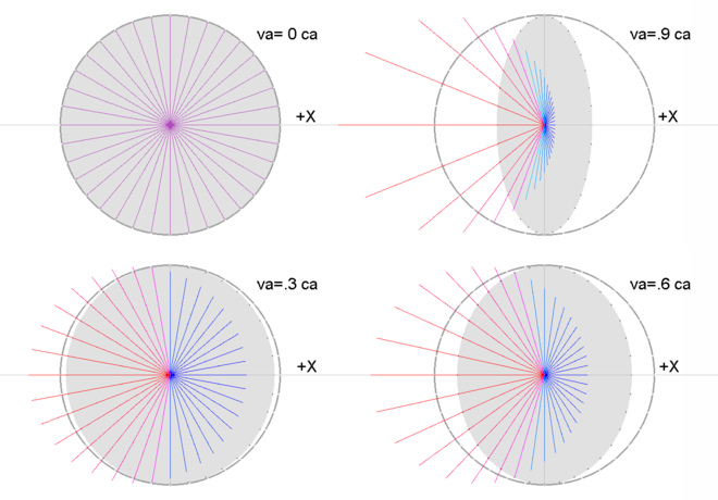 |
In each figure the oscillations are shown traveling in 36 different directions, and when the oscillations
reach the system's periphery, they are reflected back in the opposite direction. They are traveling at the
absolute speed of light, ca, through the qm, and therefore travel at various speeds through the systems moving
through the qm. The lengths of the colored lines show the speeds of the oscillations through the systems. If
the major radii of the systems are 1 , then for the system at rest in the qm
(upper left figure) the lines every 10 degrees show that the speed of light in all directions
is 1 ca. When va=.3 ca (lower left), the colored lines show the speeds of light in the system
ranging from .7 ca in the +x direction to 1.3 ca in the –x direction. The figures
show this asymmetry in the speeds of light becoming much greater as the speeds of the systems through the qm
approach the speed of light. The figures also represent systems on subatomic scales because the same
phenomena shown in the figures occur at all scales of mass/energy.
The figures show the increased energy of the blueshifted oscillations (blue) that move slower through the system,
and they show the decreased energy of the redshifted oscillations (red) that move faster through the system. The
system moving with .6 ca velocity through the qm has four times as many blueshifted oscillations
moving in the +x direction with a velocity of .4 ca through the system than it has redshifted
oscillations moving with a velocity of 1.6 ca through the system in the −x direction. When
an oscillation (e.g. photon) having an oscillation frequency of 200 Hz is moving in the +x direction
and is reflected in the opposite direction at the periphery of the system that is moving with a velocity of
.6 ca through the qm, it is Doppler redshifted by a factor of 4. The resulting 50 Hz photon
then moves in the −x direction with a velocity of 1.6 ca through the system and when it
encounters the periphery it is Doppler blueshifted back to a 200 Hz oscillation. Even in the transverse
directions in the system, the oscillations are blueshifted from the frequencies and energies they would
have if their systems were at rest in the qm. This is explained on pages 22−24 of this website. These pages
also show why the total mass/energy of all the oscillations in a system or body moving through the qm with
velocity, va, is equal to the mass/energy of the system's oscillations when va=0 ca divided by the system's
physical change ratio, rv. This correlation between absolute velocity and the mass/energy of a system's
oscillations agrees exactly with the experimental evidence. This agreement is part of the wide variety of strong
evidence supporting this view that all mass/energy is oscillations of a quantum medium.
Bicycle example:
A bicycle and rider with a total mass/energy of 70 kg will be used to analyze what occurs when this "body" is
accelerated from 0 m/s to 9 m/s (32.4 km/hr) relative to the level ground. We will first
calculate the work required to attain this 9 m/s speed. We will assume that the rider can cause a horizontal
force of 70 newtons (N) between the rear wheel and ground. (On Earth, 70 N is about the gravitational
force within 7 liters of water.) Sans friction and drag, this force will cause a 1 m/s
acceleration of the 70 kg body, and after 9 s, the body's speed will be 9 m/s, and the body will
have moved 40.5 m in 9 s with an average speed of 4.5 m/s. Therefore, the work done by the
70 N force on the body is 70 N · 40.5 m = 2835 joules (J). This is
the amount of energy required to lift the 70 kg body 4.13 m above the ground. Note that we are using
virtual units of distance, force, and mass/energy/work (i.e. m, N, J, kg) in our calculations.
These units are probably very close to absolute units (i.e. ma, Na, Ja, kga) because the sun's
absolute velocity is probably very low relative to ca.
In the context of the 2835 J of energy needed for the 9 m/s change in speed of the 70 kg
body, it is hard to believe that the body has an internal energy of 6,300,000,000,000,000,000 J,
especially when it is understood that this is the amount of energy required to lift up all the water in
Lake Baikal (23,615 km) a distance of 27 m. Why does the body have this
6.3E18 J of internal energy tied up in its atoms and smaller scale constituents? Experiments have
shown that all bodies have this huge internal energy and that a body's internal energy in J is equal to its
mass in kg times the square of the speed of light in m/s (i.e. e=m·c).
But how can mass have so much internal energy? Has there been a plausible explanation for the source of this
energy? In the qm view, the energy is contained in the oscillations of the medium that are constantly moving
in all directions through the body. (The body's 6.3E18 J of internal energy is equivalent to about
5E33 X-ray photons oscillating in the body.) It is the combined energy of the many oscillations
that cause bodies to resist changes in their velocity, as this bicycle example will show.
When the body's absolute velocity (vBa) is changed by 9 m/s (.00000003 c), this causes a change
in the speeds and energies of the oscillations moving through the body. The changes are like the changes shown in
the four figures above, but very much smaller. A 9 m/s change in vBa causes the maximum and minimum speeds
of energy through the body to change by about 3 parts in 100 million, and the changes in Doppler shifts
in the body are correspondingly small. Although the shifts are small compared with the shifts due to the velocity
differences in the figures, they nevertheless require significant work to make the change because the body
contains so much energy.
As vBa is changed by 9 m/s, the amount of work required is equal to the resulting change in the mass/energy
of the 70 kg. To simplify the discussion, we will assume that the 9 m/s or .00000003 ca change
in velocity is in the same or opposite direction as the body's absolute velocity, and we will calculate the change
in mass/energy due to the change in absolute velocity. This change in mass/energy is equal to
(70 / (1−.00000003)) − 70 or
3.15E−14 kg, which when multiplied by c is a 2835 J change in
internal mass/energy. This is the same as the 2835 J of mass/energy exchanged with the ground during the body's
acceleration. Therefore, in the qm view, when we change our velocity on a bicycle or on foot or in a motor
vehicle, we must change the oscillations and mass/energy of our system. Understanding this helps understand why
changing our velocity requires work and the exchange of mass/energy with our environment.
Pages 25−26 show that observers moving relative to a body observe a virtual mass of the body unless they
allow for the consequences of their motion and the body's motion through the quantum medium. They show why the laws
of physics agree with the observed phenomena even when observers use incorrect, virtual observations that make it
appear that a body gained mass due to an increase in its velocity relative to the observer when, in fact, the body
lost absolute mass because increasing its velocity relative to the observer resulted in decreasing its velocity
through the quantum medium.
Newton's laws of motion, and the acceleration of mass/energy
Physics textbooks today say that Newton's laws of motion are not accurate in cases involving high relative velocities.
Page 25 shows that Newton's familiar F=m·a needs to be modified as shown in the equation below, where
the unit of force, F, is the absolute newton, Na, and where m and a are also in absolute units.
This modification results in exact agreement with observed phenomena. It is important to understand that, in any
system moving through the qm, the ratio of the absolute unit of force, Na, to the virtual unit of force, N, like the
ratio of the absolute unit of distance, ma, to the virtual unit, m, depends on the direction of the force relative to
the direction of absolute velocity. For example, in a system moving with velocity .6 ca through the qm, a virtual
1 newton force, N, in the direction of absolute velocity is equal to 1 absolute newton, Na, but
in a direction transverse to the direction of absolute velocity, a 1 N force is equal to (1/rv) Na or
1.25 Na. This is explained in the qm view booklet (pages 38−39),
available by clicking here.
These pages show an example of interesting consequences of the quantum medium and the self-consistency of the
qm view.
F · rv = m · a = m · a |
Why accelerations create internal energy-exchange imbalances in bodies
It was shown above that changing a body's absolute velocity changes the pattern of energy moving within the body.
We will now discuss why the acceleration necessary to change a body's velocity causes an energy-exchange imbalance
within the body that results in a net force within the body equal to the external force causing the acceleration.
We will consider a simple example showing what, in the qm view, occurs during acceleration to cause this
internal force.
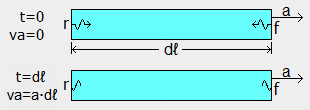
The box below is shown at two times (t=0 s and t=.000001 s). The box is
.000001 (300 m) long, and when it is at rest in the qm, the time duration
for energy quanta to travel between the ends of the box is .000001 s. To simplify this
explanation, the absolute velocity of the box will be va=0 ca at time t=0 s, when the box begins
moving through the qm due to acceleration, a, in the direction shown. Also at time t=0 s, a photon is
emitted at the front (f) of the box and a second photon is emitted at the rear (r) of the box, as
shown. The photons have the same frequency/energy and move in opposite directions. After traveling for about
d s, the photons are absorbed. Due to the acceleration of the box, the photon
arriving at r is blueshifted by a factor of (1+a·d), and the photon
arriving at f is redshifted by a factor of (1−a·d).
The rear end of the box had a net gain in energy of a·d times the emitted energy
and the front of the box lost this amount of energy. If the acceleration of the box is 30 m/s or .0000001 c/s and the box is 300 m or .000001 long, then
a·d is 1E−13. The force on the box required for this very small energy-exchange
imbalance is 30 N for every kg of mass/energy in the box, as every physics student knows.
In the following discussion of gravity, we will refer to this a·d term,
which determines the energy-exchange imbalance in the box.
or .0000001 c/s and the box is 300 m or .000001 long, then
a·d is 1E−13. The force on the box required for this very small energy-exchange
imbalance is 30 N for every kg of mass/energy in the box, as every physics student knows.
In the following discussion of gravity, we will refer to this a·d term,
which determines the energy-exchange imbalance in the box.
Physical change ratio, rg
The second of the qm view's two premises says that all systems of mass/energy affect the quantum medium in their
vicinity, and that the effects are specified by the below equation where rg is the physical change ratio
at a particular location in the quantum medium due to Earth or other concentration of mass/energy. Mass, m, is in
kga units, is the distance from m in LS units, and G is Newton's gravitational constant
(which is 2.47E−36 when distances are in LS units). At locations on or outside spherical
bodies (e.g. Earth), is the distance from the body's center of mass. All massive bodies
slow the rates of energy exchange within all systems in their vicinity in proportion to rg, and like rv, rg specifies
other characteristics of the systems. For example, all systems are contracted in all directions in proportion to rg.
A sphere that has a 1 ma diameter where rg=1 has a .9 ma diameter where rg=.9.
The following examples show some effects specified by rg.
|
rg = /( + (m·G))
or
rg = 1 / (1 + m·G/)
|
Example using rg equation to determine higher energy-exchange rate at higher elevation on Earth
A simple demonstration showing Earth's gradient of rg can be made with two atomic clocks. This example is
consistent with the known effect of Earth's mass on atomic clock rates. The rates of energy exchange within the
clocks are proportional to rg, which, like rv on Earth, is very close to 1. Therefore, the virtual distances, times,
masses, and other quantities we observe on Earth are very close to the absolute quantities. At any particular
location on Earth, rg depends on more than Earth's mass. The decrease of rg on Earth due to the sun's mass is 14
times greater than the decrease due to Earth's mass. And the mass of our galaxy probably decreases rg on Earth by
at least 2000 times the decrease caused by Earth's mass. However, Earth's mass has a much greater influence on the
gradient of rg around Earth. We can demonstrate this gradient by taking one of two clocks that are
initially located together and synchronized at sea level to a 3000 m elevation location. This change in
elevation will change rg due to Earth's mass from .9999999993056505 to .9999999993059773
or a .0000000000003268 increase in rg (assuming the following: Earth mass=5.97E24 kga,
Earth radius=.021237 LS, G=2.47E−36, and 3000 m =.00001 LS).
Therefore, if the clocks are brought together again at the end of a year (31536000 s), the clock that was at
3000 m elevation for a year will be about 10.3 microseconds (.000010306 s) ahead of the
sea-level clock. Other factors will affect the clocks' rates, the biggest factor being the higher velocity of the
3000 m clock around Earth's center, but these other factors are minor relative to the elevation change.
Example using rg equation to determine gravity on Earth
The weight of our bodies on Earth is also the result of Earth's gradient of rg (and the mass/energy of our bodies).
The gradient of rg around a massive body is responsible for the massive body's apparent "gravitational attraction,"
as explained on page 28. The gradient of rg around Earth results in a very small energy-exchange imbalance
within any system located in the gradient. Although the gradient of rg in our bodies caused by Earth is small,
the effect of the gradient is very noticeable because our bodies contain so much internal energy in constant motion
in the quantum medium. We don't sense this internal energy, so it seems incredible that a person weighing
70 kg (≈154 lb) contains the energy of 5E33 X−ray photons or enough energy
to light a 100 watt bulb for 2 billion years.
To show how Earth's mass affects our weight, we will simplify the rg equation (above-right) to the following, which
closely approximates rg around Earth because m·G/ is very small.
The difference between the calculated values of rg at Earth's surface using the rg equation above and the approximation
below is only 5E−19.
| rg ≈ 1 − m·G/ |
We can use this equation to determine how a large concentration of mass/energy (e.g. Earth) affects the transfer
or exchange of energy within every body in its vicinity. The figure shows the box with length d
now at rest in the qm and in the vicinity of a massive body, m, which is shown small and dense for convenience.
Because the rate of round-trip energy transfer and the rates of all processes are slowed in proportion to rg at their
location in the cosmos, the oscillation frequencies and energies of the photons emitted in the box are now lower than
when unaffected by mass, m. The energy of the photon emitted at the front of the box is
1−(m·G/) times its energy sans m, and the photon at the rear of the box has
1−(m·G/(+d)) times the energy sans m. Therefore, when
the photons are absorbed, there is a net gain of energy at the front of the box and a net loss at the rear.
The right side of the following equation is the energy-exchange imbalance in the box due to massive body, m, which
causes a higher value of rg and higher energy emitted at the rear of the box and a net energy-exchange imbalance
toward the front of the box. In the qm view, it is this energy-exchange imbalance within all bodies in gradients
of rg that determine their gravitational acceleration. For a body in free fall in a gradient of rg, the energy-exchange
imbalance due to the gradient of rg is equal and opposite to the energy-exchange imbalance due to the
body's acceleration in the quantum medium, as specified by the left side of the equation. In a gradient of rg, a
body accelerates in order to balance its internal energy exchange. The following equation reflects this balancing.
|
a·d = ( 1 − m·G/(+d) )
− ( 1 − m·G/ ) |
If we divide both sides of the equation by d as shown below, the right side now represents the
gradient of rg in the box, or the change in rg over the length of the box. This gradient of rg will be
represented by the symbol, rgg, as shown.
|
a = ( ( 1 − m·G/(+d) )
− ( 1 − m·G/ ) ) / d = rgg |
This equation can be simplified as follows.
a = ( m·G/ − m·G/
(+d)) / d = rgg
a = m·G/
(+·d) = rgg
G = (a/m)·(+·d)
|
In the preceding equation, we can specify values for m, , d and then either
specify G (which Newton determined empirically using other reasoning) or specify an acceleration and solve for G. If
we use Earth's 5.97E24 kg mass for m and use .021237 (6371100 m)
for Earth's radius and , and use .0000000327 ca/s
(9.81 m/s) for the free fall acceleration near Earth's surface, we can use any
value for d that is very small relative to Earth's radius because this value does not significantly
affect the value we get for G. When using d=.000001
(300 m), the calculated value for G is 2.47E−36
kg s or 6.67E−11 m
kg s.
In the rgg equations above, as d becomes very small, terms with d
become insignificant. Therefore, rgg and acceleration, a, are simply
m·G/. Because rg is approximately equal to
1−(m·G/), the first derivative of this function with respect
to specifies the approximate rate of change in rg at a given distance,
, from mass, m. This derivative is
m·G/. Therefore,
m·G/ is a good approximation of rgg when
m·G/ is very small relative to 1.
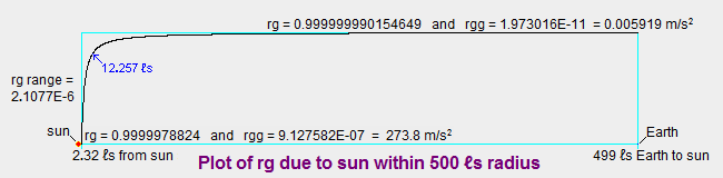
The black curve in the following image shows the relationship between rg due to the sun (red dot) and the
distance from the sun along the horizontal axis. It shows this relationship from the surface of the sun, which
is 2.32 from the sun's center, out to a distance of
499 , which is Earth's distance from the sun. It shows the value of rg and rgg at
the sun's surface and at Earth. The curve shows that the gradient of rg, and therefore the "gravitational
attraction" of the sun, changes rapidly near the sun. Although the gravitational acceleration at the sun's surface
is 28 times our gravity on Earth, at a distance of only 10 more from the sun,
the sun's gravity has decreased to our gravity on Earth. (This 12.257
location on the curve is shown by the little blue arrow.) When the curve reaches Earth's distance from the sun
it is so flat that for a body on Earth the net gravitational force within the body pushing it toward Earth's
center is about 1650 times the internal force pushing the body toward the sun. In spite of the sun's very weak
.005919 m/s gravitational acceleration at Earth, the decrease in rg
(and therefore the decrease in the rates of clocks) on Earth due to the sun's mass is 14.1 times the decrease due
to Earth's mass. This combination of the sun's substantial effect on rg on Earth and low effect on gravity on Earth
is due to the sun's low gradient of rg on Earth, as the curve shows.
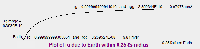
The curve below for Earth's effect on rg shows that at .25 from Earth the sun
has (1−.999999990154649) / (1−.999999999941016) or 167 times
as much influence on rg as Earth (as opposed to 14.1 times at Earth's surface). If the distance from Earth
is extended from .25 to 499 ,
Earth's effect on rg decreases to only (1−.999999999999970) or 3E−14. At this distance the sun
has a 984535E−14 effect on rg, which is 3.28178E5 times Earth's effect. Therefore, the sun's
influence on rg in the universe reaches much farther than Earth's influence, which is expected because the sun's
mass is 3.3E5 times Earth's mass. These examples help show that the qm view's simple equations and
theory provide a logical explanation for the "force of gravity," the slowing of clocks due to massive systems,
and a wide variety of other phenomena.
The above equations are in agreement with the experimental evidence and they specify the accepted
"gravitational accelerations" caused by the concentrations of mass/energy listed in the following table.
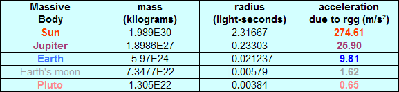 |
Because the equation g = m·G/ of orthodox
physics theory is a good approximation of rgg only when m·G/
is very small relative to 1, it is unsatisfactory for determining rgg near extremely massive and dense bodies such
as neutron stars (where m can be 3E30 kg and can be
.00004 , and m·G/
can be more than 0.2). Only in such cases where bodies are comprised of extremely dense mass/energy
do the qm view and orthodox gravity theory predict significantly different observed, virtual phenomena.
Gravity near neutron stars and black holes
The qm view specifies gravities near neutron stars that are less than the gravities specified by orthodox
Newtonian gravity. The gravitational acceleration,
g = m·G /, specified by Newton's law
is the derivative of rg≈(1−m·G/) with respect to ,
and this approximation of rg is good only when rg is close to 1. Neutron stars can result in rg being substantially
less than 1 and we can hypothesize conditions where m·G/ is greater than 1 and
rg is negative. This is equivalent to a negative energy-exchange rate and other illogical phenomena.
The acceleration, rgg, specified by the qm view is the derivative of rg=1/(1+(m·G/)),
which is rgg=m·G / ((m·G) + ).
This gradient of rg for any particular distance, ,
from source mass, m, should be a more logical basis for Newton's law of gravity than the customary
g = m·G /, which is
the derivative of an approximation having the aforesaid limitations.
Newton's law of acceleration due to gravity, specified as follows, would avoid these limitations.
|
g = m·G / ((m·G) + )
|
The difference between the acceleration at the sun's surface specified by the orthodox
Newtonian gravity equation and the modified equation above is only (275.9311 m/s/s −
275.9299 m/s/s) or .0012 m/s/s or 4E−12 ls/s/s.
But the difference near the surface of a neutron star having the sun's 2E30 kg mass and a radius of
.00004 is (3096 ls/s/s − 2451 ls/s/s) or 645 ls/s/s.
Thus, in the qm view, the acceleration predicted by current orthodox theory is 26% too large, and this
miscalculation of gravity may be causing significant errors in cosmological theory.
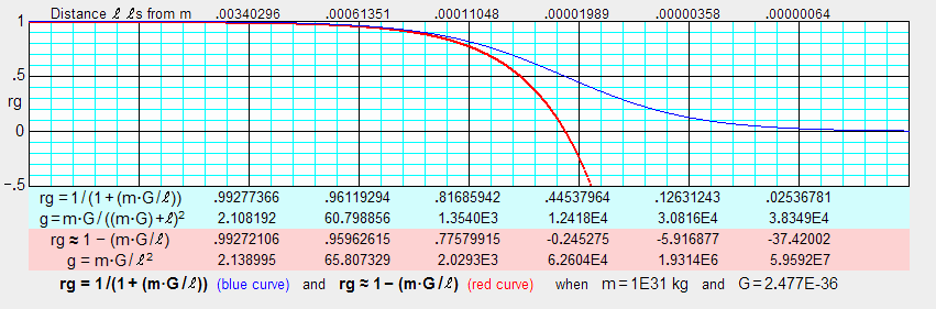
The above figure shows how the physical change ratio rg (blue curve) and the approximation
of rg (red curve) diverge significantly in extreme gravity environments.
As the text at the top and bottom of the figure indicates, the curves are for short distances
from an extremely compact 1E31 kg mass (five times the sun's mass). For each of the
distances shown (in units) at the top of the figure, rg and the
gravitational acceleration, g, are shown in the blue box under the curves, and the
approximation of rg and the orthodox value for g is shown in the red box. It can be
seen that the orthodox Newtonian gravity equation significantly understates rg and overstates
g when rg is significantly less than 1. The figure shows that the approximate rg
becomes negative at about .00002 from mass, m. In
the qm view, rg=0 means that the energy-exchange rate in a body is zero. Therefore,
a negative value for rg is probably unrealistic and incorrect for any system of mass/energy.
This discussion of gravity near dense and massive bodies has not considered the changes that
these bodies create in the mass/energy in their vicinity, including in themselves. The observable
changes include decreases in the bodies' mass/energy and their volume in proportion to rg and
rg respectively.
This discussion would be complicated and would involve some uncertainty, but we are confident that it
would not alter the conclusion that in very high gravity conditions rgg provides better predictions of
gravitational accelerations and a better explanation of the causes of the accelerations
than current orthodox Newtonian gravity theory.
Unless this thinking can be faulted, the implications of the lower gravities specified by
the modified Newtonian equation are probably significant. The realization that gravity is a
function of the gradient of rg and not a function of may help
make more sense of nature (e.g. by showing that extreme gravities that permit traveling back in time
and changing history are unrealistic, and by creating awareness of the physical causes of gravity).
Gradients of rg around massive bodies
The gradients of rg around planets or other spherical bodies are roughly symmetrical and the magnitudes and
directions of the resulting gravitational forces are easily determined. However, where two or more massive bodies
significantly influence the gradient of rg at a location in the universe (e.g. on Earth), the situation is
more complex. The qm view can probably help understand this complexity.
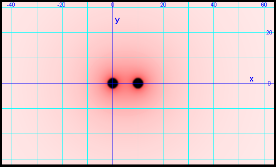
To see how massive bodies result in complex gradients of rg, we can consider two hypothetical solid spherical bodies
about as large as our sun with radii of 2.3 and masses of 2E30 kg.
The bodies are located 10 apart, as shown in the following figure. Due to the
gradient of rg between them, their acceleration toward one another is about 30 m/s.
If they are initially at rest relative to one another, they will crash together in about 2.6 hours with
a relative velocity of about 450,000 m/s. To avoid crashing (and avoid trying to explain how they could
be at rest relative to one another), we will assume they are moving relative to one another.
At any point on the coordinate system, the magnitude of the gravity caused by the gradient of rg is proportional
to the change in rg per unit distance in the coordinate system. Each pixel in the image represents a
.2 square area and the darkness of the red color of the pixel represents the
amount that rg is decreased from rg=1. Therefore, the gradient of red color shows where the
gradient of rg and the resulting gravity are higher and where they are lower. Although there is considerable
variation in the red color, the variation does not represent large changes in rg. For example, at the
(x=40 , y=30 ) location, rg is about
.999999784 and at (x=5, y=0) rg is .999998024. The gravity force within a small
body at any particular location in the gradient is proportional to the maximum gradient of decreasing rg
at the location, and the direction of the gravity force in the body is the direction of this maximum gradient.
There is no gravity at (x=5, y=0) because the gradient of rg is zero in all directions.
At any location on the coordinate system, rg is probably the product of the rg due to mass (0, 0) and rg due to
mass (10, 0), and our calculations are based on this assumption. We assume that multiplying the rg values for the
masses gives the rg value for all the masses together, regardless of the number of masses. Like other aspects of the
qm view, this may not be exactly correct, but we think it is close to correct.
Gradients of rg around massive bodies affect systems of mass/energy moving through the gradients in various ways.
They affect the motion of all energy through the quantum medium and therefore affect all mass/energy in the gradients.
The following describes how rg affects the propagation of light and all other energy quanta through the quantum medium.
Effects of rg on the speed and paths of light
In regions of the universe where rg is less than one due to the influences of concentrations of mass/energy
(probably everywhere), the speed of light through the qm is less than ca, the theoretical maximum speed of light.
At any particular location in the universe where rg<1, the speed of light is designated cag and specified by
the following equation where rg is the product of the rg for each concentration of mass/energy slowing the speed of
energy quanta through the qm at that location. For example, cag in space just beyond Earth's atmosphere is equal to
the square of the product of rg due to Earth, rg due to the sun, rg due to the rest of our galaxy, and possibly rg
due to other significant mass/energy.
cag = rg |
The gradients of rg around large concentrations of mass/energy such as Earth, the sun, and our galaxy cause the
paths of light and all energy quanta moving through the gradients to be bent, much as light is refracted when
moving through the air density gradient around Earth, but to a much smaller extent. The cag equation above and
the following dxca equation and the figure below it specify the algorithm for determining the speeds and paths
of light through gradients of rg.
| dxca = dt · (sinθ) · (1−cag) / |
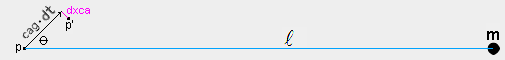 |
For example, during a small time increment, dt sa, a photon, p, which is a
distance, LS, from a massive body, m, has a velocity, cag,
specified by the cag equation. The photon moves a distance, cag·dt LS, with an initial trajectory
at angle, θ, to a line to the massive body, as shown. The photon also has a component of
motion, dxca, specified by the above equation, at right angles to its initial trajectory and toward the massive
body, as shown. These two components of motion specify the photon's location p' at the end of the time increment. A line
from p through p' specifies the initial trajectory angle for the next time increment. Using this step-and-repeat process,
a photon's motion through a gradient of rg in the qm can be computed. The simple rg, cag, and dxca equations are
consistent with the experimental evidence that has been cited to support general relativity theory.
For example, experiments using radar signals sent from Earth to Venus and back when Venus was on the far side of the
sun showed that photons traveling close to the sun are slowed due to the sun's large mass. When a round-trip
radar signal passed within about 10 LS of the sun's center, the signal was delayed by about 170
microseconds. And when a signal passed within about 120 LS of the sun, it was delayed by about 80
microseconds. The time delays specified by the above equations are 182 and 84 microseconds, in general
agreement with observations.
The bending of the paths of photons due to the sun's mass has also been determined by observing stars and quasars,
which are observed passing behind the sun as Earth revolves around the sun. The observed bending when a photon's
path just grazes the sun's surface is 1.75 arcseconds. And the observed bending when the path comes within
78 LS of the sun's center is .05 arcseconds. The bendings specified by the above equations are
1.746 and .051 arcseconds.
Influence of rg on the orbit of Mercury and other planets
The qm view explanation of the observed gravitational force has been discussed above.
And the effects of the sun's and planets'
gravities on planet orbits is well known and will not be discussed. However, we will discuss the
so-called anomalous precession of planet orbits, which has been of considerable interest to
astronomers and physicists.
For many, the fact that spacetime theory provides an explanation for the 43 arcsecond per century
anomalous precession of Mercury's orbit confirms their belief that spacetime theory accurately
represents physical reality. Many believe, incorrectly, that spacetime provides the only plausible
explanation for the anomalous precession. The qm view not only provides a simple
explanation, it also identifies the physical causes of the phenomenon.
The primary cause is the photon-slowing gradient of rg around the sun. This gradient affects the
paths of all bodies moving through the gradient because it affects the paths of the photons and all other
energy quanta moving within the bodies and moving through the qm with speed, cag. The rg, cag, and
dxca equations and figure above specify the effect of the sun on a planet's energy quanta that comprise
the planet's entire mass/energy. Because a planet's energy quanta are the planet, how they move
through the qm determines how the planet moves. This, and the resulting anomalous precession of
planet orbits, are explained
here.
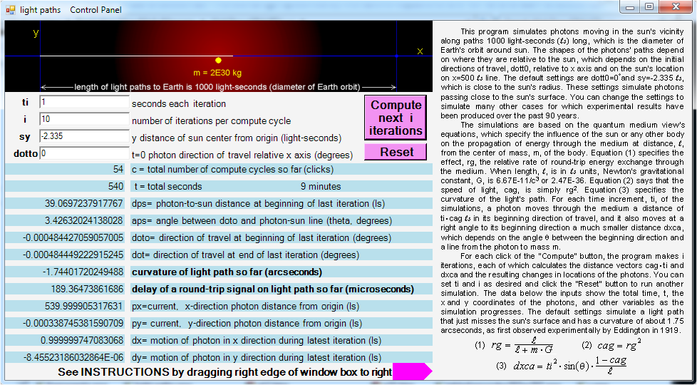
Computer program for showing sun's influence on the speed and paths of light
The image below shows the control panel of a computer program that calculates the slowing of light and the bending
of light paths around the sun due to the gradient of rg caused by the sun (represented by yellow disc). The image
shows the path of a photon (white line) during the first 540 seconds of travel along a 1000 light-second path
that grazes the sun's surface. It shows that the "Compute next i iterations" button has been clicked 54 times and
that each click resulted in 10 iterations of the algorithm, and that the time increment, ti, for each
iteration is 1 second, so that a total of 1x10x54 or 540 seconds or 9 minutes have elapsed. (Please note that
symbol, ti, and symbol, dt, in the above dxca equation both mean the time increment.) The image shows
that, during the 9 minutes of photon travel, the trajectory angle has decreased by .000484449 degrees, which
is 1.7440 arcsecond of curvature of the photon's path, which agrees with experimental evidence.
The simulation also shows the slowing of the photons, multiplied by 2 so it shows the slowing of a radar signal
making a round trip from Earth and passing near the sun. By changing the sy input in the third box on the
control panel, the photon path can be made to pass other distances from the sun's center to show that the slowings
are also consistent with other experiments.
Instructions for using this program are revealed by dragging the right edge of the control panel to the right,
as shown. This computer program helps understand the small-but-far-reaching effects of large concentrations of
mass/energy on the propagation of energy through the qm. In the qm view, these effects are also responsible for
gravity and other related phenomena as discussed elsewhere on this website and in the qm videos. This
Visual Basic (.exe) program is 136 Kb and if you want to download and experiment with it,
click here.
Note: Depending on your computer security system, you may get a warning that this program
can harm your computer. We have been assured by our security provider (Frontier Secure of Frontier Communications)
that this program, of our own making, is not a threat to any computer. Therefore, please be assured that it
is safe to authorize your computer to run this program.
The qm view leads to other equations and other modifications of equations such as F=m·a, but
the above equations permit a good understanding of the qm view. We think that the equations and qm view are
probably a correct representation of nature for the following reasons. They are consistent with the experimental
evidence and explain physical causes for the wide range of phenomena they predict. They are relatively simple,
as you can see. They explain phenomena that orthodox theory cannot explain (e.g. constant light speed, c, and the
source of the energy and inertia of matter). They are based on two logical premises that lead to logical conclusions
without paradoxes and without having to adopt an artificial system of spacetime due to assuming constant light
speed, c. If you think otherwise, or have questions or suggestions, we can be reached
here.
To return to qm view, close tab or browser 
|
|