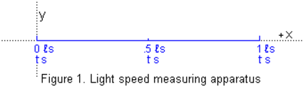
The apparatus:  A large apparatus for measuring the speed of light is shown in Figure 1.  It consists of a rigid scale having a length of 1 light-second (1 ), and it has an x,y,z coordinate system, the x axis of which is coincident with the long axis of the scale, as shown.  It is floating freely in remote space and has no rotation relative to the observed universe.  At the x=0  location, a shutter can be opened to allow light that is arriving from the −x direction to travel to the x=1  location where a light detector and a mirror can detect and reflect the incoming light back to the x=0 location, which also has a detector and mirror.  Both locations also have atomic clocks and radio transmitters and receivers to communicate the times of events such as shutter opening and light receiving.


The 1  length of the apparatus, the .5  location, and the synchronization of the clocks (as shown) can all be established and confirmed by broadcasting from the x=.5  location a signal containing the time, to, on clock x=.5 when the signal is broadcast.  Then, when the signal, to, arrives at clocks x=0 and x=1, these clocks should read exactly (to+.5) s as the signal is reflected back to x=.5 where the returning signals should arrive at exactly (to+1) s on clock x=.5.

Using the apparatus to measure light speed:   Observers aboard the apparatus use it to confirm that the speed of the incoming photons from a light source is always the same speed, c.  For example, they can maneuver the apparatus to align it with a star or other distant light source in the −x direction and then allow the apparatus to float with this constant orientation in its inertial reference frame.

Then, when the shutter at x=0 is quickly opened, photons from the star begin traveling to the mirror at x=1 where they are reflected back to the receiver at x=0.  The elapsed time according to the x=0 clock is always exactly 2 s.  Also, according to the synchronized clocks, the travel time for the starlight moving in either direction between x=0 and x=1 is always 1 s.  Furthermore, the observed measurements of light speed, c, are not affected by the velocity of the apparatus toward or away from the source (which velocity the observers can determine via the observed blue or red shift of the incoming light).  This description of how light speed, c, can, in theory, be confirmed is consistent with current orthodox physics theory.

The qm view explanation of observed light speed, c  
The observers aboard the apparatus do not realize that light in their vicinity is propagated with a constant absolute speed, ca, through a quantum medium, qm.  (Even in Earth's atmosphere, the speed of light through the qm is only slightly less than ca.)  This results in the speed of light being anisotropic for any body or system of mass/energy (e.g. the apparatus or sun) that is moving through the qm.  When the apparatus system is moving through the qm with an absolute velocity, va, as shown in Figure 2, this velocity through the qm slows the rate of round-trip energy exchange in the system, which slows all clocks and other processes, and causes clocks that are virtually synchronized to be absolutely asynchronized.  The absolute velocity, va, also causes the apparatus to contract along lines parallel to va, which keeps the rates of round-trip energy exchange within the apparatus isotropic (as they are when va=0).  These phenomena, which are all logical consequences of a quantum medium, are explained in detail at the qm view website.

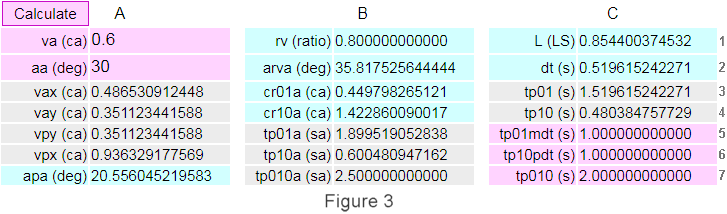
To show why experiments always measure light speed, c, we will use an example corresponding to Figure 2.  As shown, the example assumes that the apparatus has an absolute velocity (i.e. through the qm) of .6 ca (where ca is the speed of light through the qm).  Also, Figure 2 shows that the direction of this velocity is aa=30 degrees relative to a blue, dashed line that represents a 1  long apparatus at rest in the qm.  Because this blue-dashed apparatus is at rest in the qm, the 1  length observed aboard the apparatus is also its absolute length of 1 LS in the qm.  Figure 2 also shows this at-rest apparatus located diagonally between opposite corners of a rigid rectangle.  And it shows that when this framework and apparatus within it are moving through the qm with velocity va=.6 ca, the framework and apparatus contract as shown by the solid lines.
Physical changes in the apparatus system:   The apparatus and rectangular framework, moving through the qm with velocity va=.6 ca, are contracted to .8 times their at-rest size along lines parallel to va.  This contraction is specified by the physical change ratio, rv, which is rv=(1−va^2)^.5 = .8.  The framework is therefore contracted from its at-rest length of cos(aa) absolute light-second, LS, (i.e. .866025 LS) to .8 · cos(aa) LS (i.e. .692820 LS).  The contracted length of the apparatus is therefore L=( (sin(aa))^2 + (rv·cos(aa))^2 )^.5 = .85440037 LS, although the observers on the apparatus who assume light speed, c, will observe a length of one virtual light-second (i.e. 1 ).

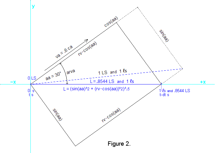
Figure 3 is a picture of the calculator at the bottom of this webpage.  The calculator determines the values for rv and L in the two equations above, and it displays the values in cells B1 and C1.  The calculator also solves all the other equations we will discuss below.  The picture shows that in the two light-magenta "input cells," A1 and A2, we have entered .6 ca for the velocity, va, of the apparatus and 30 degrees for the angle of the velocity relative to the apparatus in the at-rest reference frame.  It shows that when va=.6 ca, the contraction of the apparatus along lines parallel to va causes the absolute angle between va and the x axis of the apparatus to be arva=35.8175 degrees (as shown in the light-cyan data cell B2).


We will now explain how each of the numbers in the cells are calculated and how they always combine to cause the observed 1 second time for light traveling from x=0 to x=1 and from x=1 to x=0, and the 2 second time for light traveling from x=0 to the mirror at x=1 and back to x=0.  These times are shown in the magenta cells in column C of the calculator.

The rationale and equations for calculating rv and L in the top row were explained above.  Similarly, angle arva in the second row is a function of the distances shown in Figure 2.  For example, arva=atan(sin(aa) / (rv · cos(aa))).

Calculating the speeds of light along the apparatus:  Figure 2 shows the x axis of the apparatus momentarily coincident with the x axis (cyan color) of a reference frame at rest in the qm.  This will make it easy to determine the direction of travel through the qm of the photons moving along the x axis of the apparatus.  We know that in the qm frame the apparatus has an x-direction velocity component, vax=va · cos(arva), and a y-direction velocity component, vay=va · sin(arva).  These equations yield the results shown in calculator cells A3 and A4.

And we know that photons moving along the x axis of the apparatus must have a y-direction velocity component through the qm, vpy, so that vpy=vay.  Therefore, the x-direction velocity component of the photons must be vpx=(1−vpy^2)^.5 because the two components result in a photon velocity of 1 ca.  And knowing vpx and vpy permits the absolute angle, apa, of photon travel relative to the x axis of the qm coordinate system to be calculated because apa=atan(vpy / vpx).  The calculated values of vpy, vpx, and apa are shown in A5, A6, and  A7.

The data in B3 and B4 show the absolute relative velocities of the photons moving along the apparatus.  The equation for calculating the absolute relative velocity of photons moving from x=0 to x=1 is cr01a=vpx−vax and the equation for photons moving from x=1 to x=0 is cr10a=vpx+vax.  As you can see, the photon speed toward x=0 is several times the speed toward x=1.

Calculating the absolute and virtual times for light to traverse the apparatus:  Knowing these absolute relative velocities and the absolute length of the apparatus, we can calculate the absolute times for photons to traverse the apparatus.  In the +x direction the travel time for the photons is tp01a=L / cr01a, and in the −x direction it is tp10a=L / cr10a.  As shown in B5, B6, and  B7, the travel time in the +x direction is about three times the −x direction time, and the round-trip time is 2.5 sa, which is 2 s on the atomic clocks because they are slowed to .8 times their at-rest rate due to va=.6 and rv=.8.  Therefore, the observed round-trip travel time, tp010, shown in C7, is exactly what the observers expect.

Time aboard the apparatus, which is specified by the atomic clocks, advances at only .8 times the absolute, at-rest rate, as discussed above.  Therefore, the clocks advance only .8 times the tp01a and tp10a absolute times for the photons to traverse the apparatus.  The lower clock times tp01=rv · tp01a and tp10=rv · tp10a are shown in C3 and  C4.

A key reason for the observers on the apparatus observing that photons take exactly 1 s to traverse the length of the apparatus in either direction is that the clocks at x=0 and x=1 are virtually synchronized, but not absolutely synchronized.  For example, if the observers at x=0 and x=1, who assume constant light speed, c, synchronize their clocks by setting them to to+.5 s when the to signal is received, the clocks will not be synchronized unless the speeds of light along the x axis are the same in both directions.  This equal relative light speed, cr01a=cr10a, occurs only when the apparatus is at rest in the qm or when the direction of va is perpendicular to the apparatus distance scale.  A simple rule for determining the asynchronization of two clocks in a reference frame moving through the qm is as follows.

RULE:  In any inertial reference frame moving through the qm, two clocks which have been virtually synchronized are out of sync by an amount equal to the absolute velocity of the reference frame times the observed distance (not LS) between the clocks in the direction of absolute motion.  The forward clock is retarded relative to the rearward clock.

In our example, the absolute velocity is .6 ca and the observed distance is cos(30) or .8660254, so the asynchronization of the clocks, dt, is .519615, as shown in  C2.  Thus, dt=va · cos(aa), (and when aa>90, then dt= −va·cos(aa)).  The clocks at x=0 and x=1 are out of absolute synchronization by an amount dt.  When an observer at x=1 gets a time-encoded signal from x=0, the observer expects the encoded time to be 1 s prior to the arrival time on the x=1 clock.  If the encoded signal is sent at to s on the x=0 clock, then the arrival time on the x=1 clock will be (to+tp01−dt) s, which observers at x=1 expect to be (to+1) s.  C5 contains tp01mdt=(tp01−dt), and C6 contains tp10pdt=(tp10+dt).  If these times are close to 1 s, they will make it appear that the travel time for light in either direction between x=0 to x=1 is 1 s.

Summary:   According to the qm view, the virtual, measured speed of light, c, is the result of absolute phenomena that have not been apparent.  The qm view specifies these absolute phenomena and explains their physical causes in detail (at the qmview.net website and elsewhere).

The qm view shows that light speed, c, is not a simple phenomenon.  Perhaps the complexity is a reason why the causes of this phenomenon have remained a mystery for so long and why people were willing to assume that constant light speed is simply a strange fact of nature.

Light speed, c, is a logical consequence of a quantum medium in which all the mass/energy of the universe exists in the form of oscillations and systems of oscillations of the qm.  This medium may be the same physical entity as the quantum vacuum assumed by quantum mechanics theory, within which quanta of energy constantly materialize and disappear.

Why do the math calculations always result in constant light speed?  Is it just coincidence?  It follows from the simple premise that all mass/energy is the result of oscillations of a qm.  The consequences of this premise not only explain c, they explain inertia, the huge amount of energy in matter, and a wide range of other important phenomena.  If this is a coincidence, and light speed, c, and the other phenomena have some other cause, it is a highly unlikely coincidence.  Therefore, we think it is very likely that the qm view explanation of these phenomena is the correct explanation.  However, we will continue to look for any problem with the qm view, and ask anyone with information that casts doubt on the qm view to bring it to our attention.

Calculating light speed, c, and its causes:   The following calculator permits readers to experiment with different absolute velocities, va, and absolute angles, aa, of their choosing to see how these variables affect the length of the apparatus, L, the rates of the clocks, rv, and the absolute speeds of light, cr01a and cr10a, along the apparatus.  By changing the values for va and aa in the A1 and A2 input cells and clicking Calculate, you can experiment with different combinations of these variables, which helps understand the qm view and physical causes for light speed, c, and related phenomena.